Deconvolution Systems Design#
In this example we explore how the various deconvolution parameters, which we learned about in previous notebooks combine to affect deconvolution results. We will create a simulated image which we will use as a test image for both deconvolution and deep learning restoration.
Design trade-offs#
Iterations - more iterations provide a better result up to a point of diminishing returns. How do we know when to stop?
PSF size - Using a larger PSF may improve deconvolution quality by increasing the spatial extent of the deblurring. However a larger PSF size requires larger borders and larger overlap between chunks. Note that the PSF size may be ‘infinite’ in thoeory (light from an emitter can propagate forever) however PSFs used for deconvolution are finite. Thus the size of PSF used for deconvolution becomes a design parameter.
Regularization - regularization can reduce noise in the output at a cost of slightly increased speed. How do we know what regularization factor to use? For the total variation regularization it is recommended to use values between 0.0001 and 0.005 see this paper but the exact value can depend on the SNR of the image.
PSF - The quality of the Point Spread Function can affect final results. If using a theoretical PSF we need to make sure the parameters used to generate the PSF match the true system parameters.
Overlap - Larger overlaps will reduce artifacts, but increase processing time and memory by increasing the size of each chunk.
Simulation#
In this example we do the following.
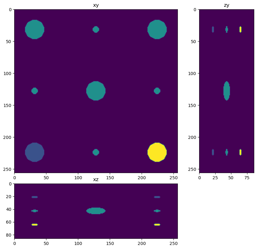
Create a simulated image with a large sphere at the center and small spheres on the sides. This sample is useful to study chunking artifacts because the chunks will subdivide the spheres.
Convolve a PSF with the simulated image and add noise.
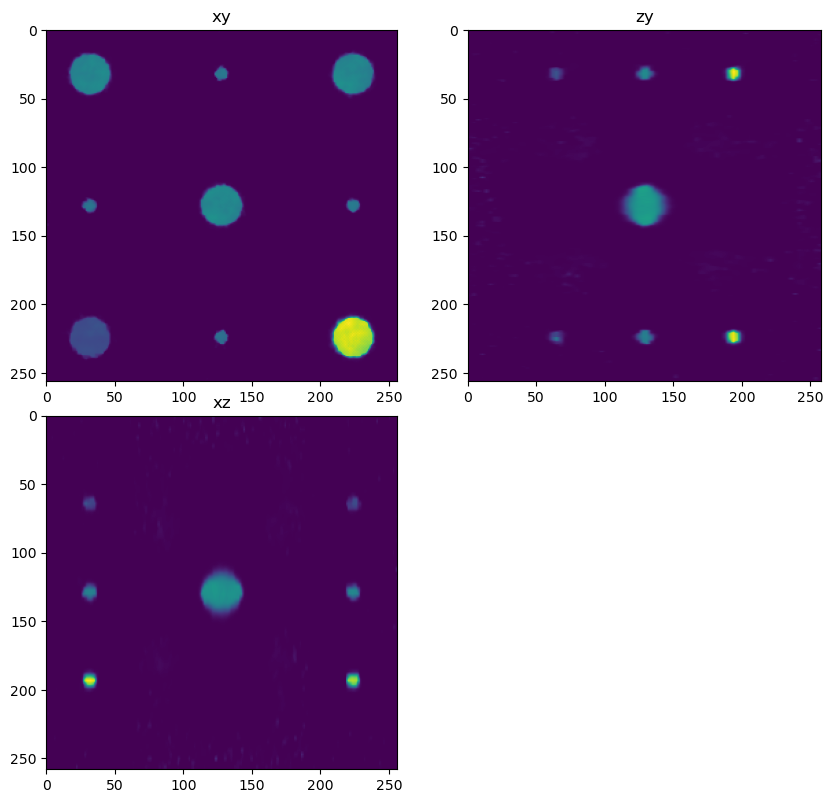
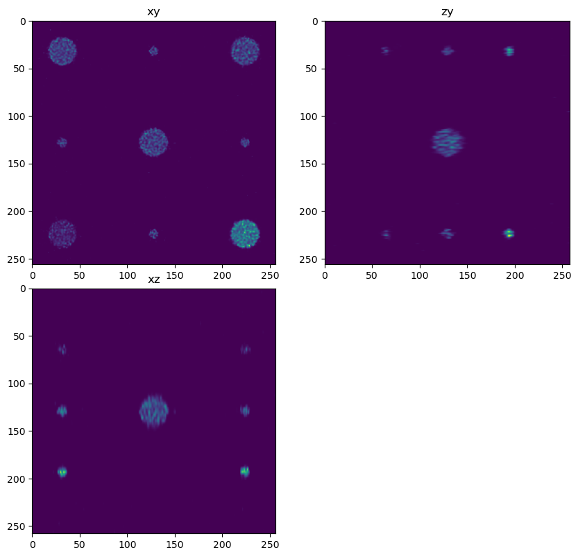
Define our deconvolution parameters including PSF parameters, dask parameters, iterations and regularization factor then deconvolve. We generate 2 deconvolutions. One with poor parameters (deconvolution PSF different than forward PSF, low iterations, no regularization, no overlap between subvolumes) and one with better parameters (deconvolution PSF = forward PSF, high iterations, overlap between sub-volumes and regularization used).
Imports#
import dask.array as da
from clij2fft.richardson_lucy import richardson_lucy_nc
import numpy as np

import sys
sys.path.append('../')
import decon_helper as dh

from tnia.deconvolution.forward import forward
from tnia.plotting.projections import show_xyz_slice, show_xyz_max
tnia available
stackview available
Create the phantom#
import raster_geometry as rg
from tnia.simulation.phantoms import add_small_to_large

gain = 400
background = 0

zdim = 256
ydim = 256
xdim = 256

phantom = np.zeros((zdim,ydim,xdim), dtype=np.float32)

r=50
r_small=5
r_medium=15
size = [2*r, 2*r, 2*r]
size_small = [2*r_small, 2*r_small, 2*r_small]
size_medium = [2*r_medium, 2*r_medium, 2*r_medium]

sphere = rg.sphere(size, r).astype(np.float32)
small_sphere = rg.sphere(size_small, r_small).astype(np.float32)
medium_sphere = rg.sphere(size_medium, r_medium).astype(np.float32)

x=100
y=100
z=50

'''
add_small_to_large(phantom, medium_sphere, phantom.shape[2]//2, phantom.shape[1]//2, phantom.shape[0]//2)

add_small_to_large(phantom, medium_sphere, phantom.shape[2]//8, phantom.shape[1]//8, phantom.shape[0]//2)
add_small_to_large(phantom, medium_sphere, phantom.shape[2]//8, 7*phantom.shape[1]//8, phantom.shape[0]//2)
add_small_to_large(phantom, medium_sphere, 7*phantom.shape[2]//8, phantom.shape[1]//8, phantom.shape[0]//2)
add_small_to_large(phantom, medium_sphere, 7*phantom.shape[2]//8, 7*phantom.shape[1]//8, phantom.shape[0]//2)

add_small_to_large(phantom, small_sphere, phantom.shape[2]//8, phantom.shape[1]//2, phantom.shape[0]//2)
add_small_to_large(phantom, small_sphere, 7*phantom.shape[2]//8, phantom.shape[1]//2, phantom.shape[0]//2)
add_small_to_large(phantom, small_sphere, phantom.shape[2]//2, phantom.shape[1]//8, phantom.shape[0]//2)
add_small_to_large(phantom, small_sphere, phantom.shape[2]//2, 7*phantom.shape[1]//8, phantom.shape[0]//2)

add_small_to_large(phantom, 1.4*small_sphere, phantom.shape[2]//8, phantom.shape[1]//2, phantom.shape[0]//4)
add_small_to_large(phantom, 1.6*small_sphere, 7*phantom.shape[2]//8, phantom.shape[1]//2, phantom.shape[0]//4)
add_small_to_large(phantom, 1.2*small_sphere, phantom.shape[2]//2, phantom.shape[1]//8, phantom.shape[0]//4)
add_small_to_large(phantom, 1.6*small_sphere, phantom.shape[2]//2, 7*phantom.shape[1]//8, phantom.shape[0]//4)

add_small_to_large(phantom, 1.1*small_sphere, phantom.shape[2]//8, phantom.shape[1]//2, 3*phantom.shape[0]//4)
add_small_to_large(phantom, 1.8*small_sphere, 7*phantom.shape[2]//8, phantom.shape[1]//2, 3*phantom.shape[0]//4)
add_small_to_large(phantom, 1.5*small_sphere, phantom.shape[2]//2, phantom.shape[1]//8, 3*phantom.shape[0]//4)
add_small_to_large(phantom, .8*small_sphere, phantom.shape[2]//2, 7*phantom.shape[1]//8, 3*phantom.shape[0]//4)
'''
add_small_to_large(phantom, medium_sphere, phantom.shape[2]//2, phantom.shape[1]//2, phantom.shape[0]//2)

add_small_to_large(phantom, medium_sphere, phantom.shape[2]//8, phantom.shape[1]//8, phantom.shape[0]//2)
add_small_to_large(phantom, 0.5*medium_sphere, phantom.shape[2]//8, 7*phantom.shape[1]//8, phantom.shape[0]//2)
add_small_to_large(phantom, medium_sphere, 7*phantom.shape[2]//8, phantom.shape[1]//8, phantom.shape[0]//2)
add_small_to_large(phantom, 2*medium_sphere, 7*phantom.shape[2]//8, 7*phantom.shape[1]//8, phantom.shape[0]//2)

add_small_to_large(phantom, small_sphere, phantom.shape[2]//8, phantom.shape[1]//2, phantom.shape[0]//2)
add_small_to_large(phantom, small_sphere, 7*phantom.shape[2]//8, phantom.shape[1]//2, phantom.shape[0]//2)
add_small_to_large(phantom, small_sphere, phantom.shape[2]//2, phantom.shape[1]//8, phantom.shape[0]//2)
add_small_to_large(phantom, small_sphere, phantom.shape[2]//2, 7*phantom.shape[1]//8, phantom.shape[0]//2)

add_small_to_large(phantom, 0.5*small_sphere, phantom.shape[2]//8, phantom.shape[1]//2, phantom.shape[0]//4)
add_small_to_large(phantom, 0.5*small_sphere, 7*phantom.shape[2]//8, phantom.shape[1]//2, phantom.shape[0]//4)
add_small_to_large(phantom, 0.5*small_sphere, phantom.shape[2]//2, phantom.shape[1]//8, phantom.shape[0]//4)
add_small_to_large(phantom, 0.5*small_sphere, phantom.shape[2]//2, 7*phantom.shape[1]//8, phantom.shape[0]//4)

add_small_to_large(phantom, 2*small_sphere, phantom.shape[2]//8, phantom.shape[1]//2, 3*phantom.shape[0]//4)
add_small_to_large(phantom, 2*small_sphere, 7*phantom.shape[2]//8, phantom.shape[1]//2, 3*phantom.shape[0]//4)
add_small_to_large(phantom, 2*small_sphere, phantom.shape[2]//2, phantom.shape[1]//8, 3*phantom.shape[0]//4)
add_small_to_large(phantom, 2*small_sphere, phantom.shape[2]//2, 7*phantom.shape[1]//8, 3*phantom.shape[0]//4)

phantom = phantom[::3,:,:]
phantom = phantom*gain
dh.show_xyz_slice(phantom, 'tnia')
# set title
#fig.suptitle('Phantom with z sub-sampling=3')
Create the forward PSF and deconvolution PSF#
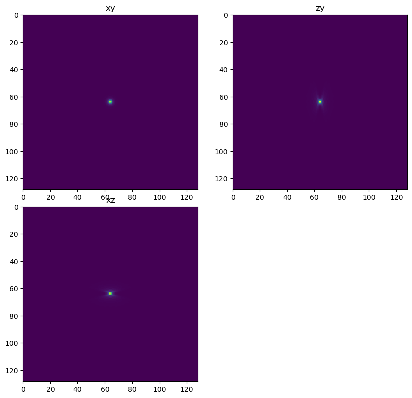
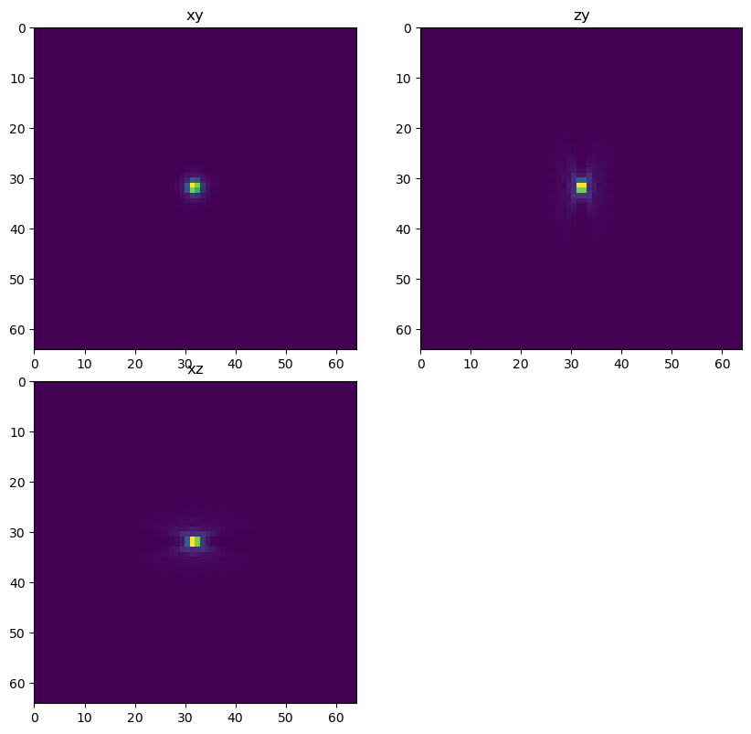
Note that the forward PSF (the PSF that explains the image) is not equal to the digital PSF used for deconvolution. Among other imperfect approximations the PSF used for deconvolution can have smaller spatial extent. In this simulation the PSF we use for convolution (ie in the simulation) is different than the PSF used for deconvolution. We can change the parameters of the deconvolution PSF to study how differences between the real PSF and the digital PSF we use for deconvolution affects the result.
Two factors which are important but may also be only approximately known are the refractive index of the biological sample and the depth of the sample (below the cover lens). These two factors combine to produce spherical aberration in the PSF.
If there is aberration in the true PSF of the system, to get a good deconvololution result that aberration must be matched in the sample.
from tnia.deconvolution.psfs import gibson_lanni_3D

x_voxel_size = 0.1
z_voxel_size=0.3

sxy = 1
sz = z_voxel_size/x_voxel_size

xy_psf_dim_forward=128
z_psf_dim_forward=128

xy_psf_dim_decon=64
z_psf_dim_decon=64

NA=1.4

# ni is the refractive index of the immersion medium of the lens
ni=1.5
# ns is the refractive index of the sample
ns=1.33

# depth at which to calculate the PSF (note if there is a RI mismatch between the lens RI and sample RI spherical aberration will be introduced
# which will be depth dependent)
#depth_forward = 10
depth_forward = 0
depth_decon = 0

psf_forward  = gibson_lanni_3D(NA, ni, ns, x_voxel_size, z_voxel_size, xy_psf_dim_forward, z_psf_dim_forward, depth_forward, 0.5, False, True)
psf_forward = psf_forward.astype('float32')
psf_forward = psf_forward/psf_forward.sum()
dh.show_xyz_slice(psf_forward, 'tnia')

psf_decon  = gibson_lanni_3D(NA, ni, ns, x_voxel_size, z_voxel_size, xy_psf_dim_decon, z_psf_dim_decon, depth_decon, 0.5, False, True)
psf_decon = psf_decon.astype('float32')
psf_decon = psf_decon/psf_decon.sum()
dh.show_xyz_slice(psf_decon, 'tnia')
Apply the forward model#
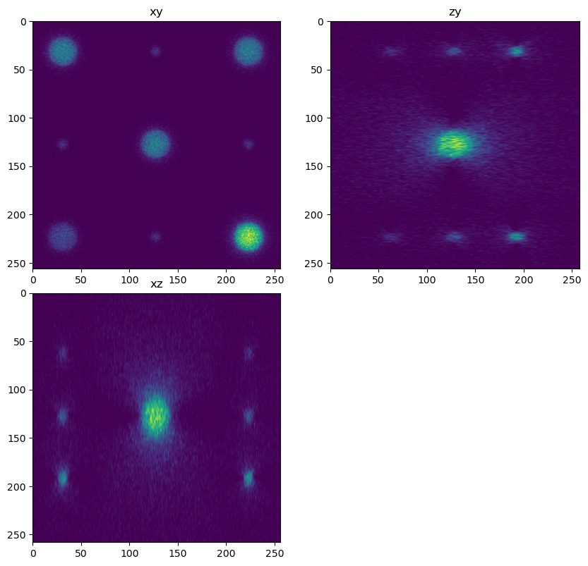
In this case the forward model is convolution with the PSF and the addition of Poisson noise.
What other factors will cause error between the true shape of the sample and the acquired image?
from tnia.deconvolution.forward import forward
from tnia.nd.ndutil import centercrop

im = forward(phantom, psf_forward, background, True, True)

x_v = im.shape[2]//2
y_v = im.shape[1]//2
z_v = im.shape[0]//2

phantom=phantom+background

fig = show_xyz_slice(im, x_v, y_v, z_v, sxy=sxy, sz=sz)
from skimage.io import imsave

imsave('../../data/deep learning testing/ground truth/spheres4.tif', phantom)
imsave('../../data/deep learning testing/inputs/spheres4.tif', im)
C:\Users\bnort\AppData\Local\Temp\ipykernel_14720\2493545118.py:3: UserWarning: ../../data/deep learning testing/ground truth/spheres4.tif is a low contrast image
  imsave('../../data/deep learning testing/ground truth/spheres4.tif', phantom)
Define number of chunks#
Define the number of chunks to divide the image into.
(In this example the image is relatively small so likely the image and arrays needed for FFT based calculations would fit into the GPU without chunking, in a real life example we would pre-compute the largest chunk size we could process given memory constraints and base the chunk size on that).
num_x_chunks = 2
num_y_chunks = 2
num_z_chunks = 1

z_chunk_size = im.shape[0]
y_chunk_size = int(im.shape[1]/num_x_chunks)
x_chunk_size = int(im.shape[2]/num_y_chunks)
print('chunks', z_chunk_size, y_chunk_size, x_chunk_size)
chunks 86 128 128
Define the deconvolver#
Define either a clij2fft based, or if clij2fft is not installed a redlionfish based Richardson Lucy deconvolution function. We map both libraries to the same deconvolution interface to make it easier to call either version in the dask step.
try:
    from clij2fft.richardson_lucy import richardson_lucy_nc
    def deconv_chunk(img, psf, iterations=100, reg=0):
            print('iterations+reg',iterations, reg)
            print('deconvolving chunk with size',img.shape)
            result = richardson_lucy_nc(img, psf, iterations, reg)
            print('/nfinished decon chunk')
            return result
            #return stack
    print('clij2fft non-circulant rl imported')
except ImportError:
    print('clij2fft non-circulant rl not imported')
    try:
        import RedLionfishDeconv as rl
        print('redlionfish rl imported')
        def deconv_chunk(img, psf, iterations, reg):
            print(img.shape,psf_decon.shape)
            result = rl.doRLDeconvolutionFromNpArrays(img, psf, niter=iterations, method='gpu', resAsUint8=False )
            print('finished decon chunk')
            return result
    except ImportError:
        print('redlionfish rl not imported')
clij2fft non-circulant rl imported
Deconvolve in chunks#
Here we call the dask deconvolution using an overlap factor to prevent edge artifacts between chunks. We try both of a set of sub-optimal parameters, and a set of better parameters to study how different settings affect deconvolution quality.
Note: Depending on the GPU memory available you may or may not need to process using Chunks. However the purpose of the notebook is to examine how various settings (including chunking settings) affect the deconvolution result, so that when we do have very large image sizes, and have to use chunking, we understand how to use chunks optimally.
#overlap = 0
overlap = 25

dimg = da.from_array(im,chunks=(z_chunk_size, y_chunk_size, x_chunk_size))
out1 = dimg.map_overlap(deconv_chunk, depth={0:0, 1:overlap, 2:overlap}, dtype=np.float32, psf=psf_decon, iterations=200, reg=0.005)
decon1 = out1.compute(num_workers=1)

out2 = dimg.map_overlap(deconv_chunk, depth={0:0, 1:overlap, 2:overlap}, dtype=np.float32, psf=psf_forward, iterations=500, reg=0.005)
decon2 = out2.compute(num_workers=1)

out3 = dimg.map_overlap(deconv_chunk, depth={0:0, 1:overlap, 2:overlap}, dtype=np.float32, psf=psf_forward, iterations=500, reg=0)
decon3 = out3.compute(num_workers=1)

fig = show_xyz_slice(decon1, x_v, y_v, z_v, sxy=sxy, sz=sz)
fig = show_xyz_slice(decon2, x_v, y_v, z_v, sxy=sxy, sz=sz)
fig = show_xyz_slice(decon3, x_v, y_v, z_v, sxy=sxy, sz=sz)
iterations+reg 200 0.005
deconvolving chunk with size (0, 0, 0)
iterations+reg 200 0.005
deconvolving chunk with size (86, 153, 153)
get lib
/nfinished decon chunk
iterations+reg 200 0.005
deconvolving chunk with size (86, 153, 153)
get lib
/nfinished decon chunk
iterations+reg 200 0.005
deconvolving chunk with size (86, 153, 153)
get lib
/nfinished decon chunk
iterations+reg 200 0.005
deconvolving chunk with size (86, 153, 153)
get lib
/nfinished decon chunk
iterations+reg 500 0.005
deconvolving chunk with size (0, 0, 0)
iterations+reg 500 0.005
deconvolving chunk with size (86, 153, 153)
get lib
/nfinished decon chunk
iterations+reg 500 0.005
deconvolving chunk with size (86, 153, 153)
get lib
/nfinished decon chunk
iterations+reg 500 0.005
deconvolving chunk with size (86, 153, 153)
get lib
/nfinished decon chunk
iterations+reg 500 0.005
deconvolving chunk with size (86, 153, 153)
get lib
/nfinished decon chunk
iterations+reg 500 0
deconvolving chunk with size (0, 0, 0)
iterations+reg 500 0
deconvolving chunk with size (86, 153, 153)
get lib
/nfinished decon chunk
iterations+reg 500 0
deconvolving chunk with size (86, 153, 153)
get lib
/nfinished decon chunk
iterations+reg 500 0
deconvolving chunk with size (86, 153, 153)
get lib
/nfinished decon chunk
iterations+reg 500 0
deconvolving chunk with size (86, 153, 153)
get lib
/nfinished decon chunk

imsave('../../data/deep learning testing/deconvolutions/spheres4.tif', decon2)
Look at error#
from tnia.metrics.errors import RMSE

print('RMSE (phantom, phantom)', RMSE(phantom, phantom))
print('RMSE (phantom, im)', RMSE(phantom, im))
print('RMSE (phantom, decon 1)', RMSE(phantom, decon1))
print('RMSE (phantom, decon 2)', RMSE(phantom, decon2))
print('RMSE (phantom, decon 2)', RMSE(phantom, decon3))
RMSE (phantom, phantom) 0.0
RMSE (phantom, im) 30.721592
RMSE (phantom, decon 1) 19.471014
RMSE (phantom, decon 2) 8.962998
RMSE (phantom, decon 2) 15.717233
Segment the spheres#
# import otsu
from skimage.filters import threshold_otsu
from skimage.measure import label, regionprops

def segmenter(im, min_area=0):

    binary = im>threshold_otsu(im)
    labels = label(binary)

    # get the regions
    object_list = regionprops(labels,im)

    filtered_objects = []
    labels_filtered = np.zeros_like(labels)

    if min_area==0:
        return object_list, labels

    else:
        for obj in object_list:

            if obj.area > min_area:
                labels_filtered[labels==obj.label]=obj.label
                filtered_objects.append(obj)
        return filtered_objects, labels_filtered
objects_truth, labels_truth = segmenter(phantom, 20)
objects_im, labels_im = segmenter(im, 20)
objects_decon1, labels_decon1 = segmenter(decon1, 20)
objects_decon2, labels_decon2 = segmenter(decon2, 20)

print('objects_truth', len(objects_truth))
print('objects_im', len(objects_im))
print('objects_decon', len(objects_decon1))
print('objects_decon', len(objects_decon2))
objects_truth 12
objects_im 13
objects_decon 12
objects_decon 12
Make figures of segmentations#
from tnia.plotting.projections import show_xy_xz_slice
from tnia.plotting.projections import show_xy_xz
from matplotlib import pyplot as plt

from tnia.plotting.projections import show_xy_zy_slice
from tnia.plotting.plt_helper import random_label_cmap

def makefigs():
    fig1=show_xy_xz_slice(labels_im, x_v, y_v, z_v, sxy=sxy, sz=sz,figsize=(4,9), colormap=random_label_cmap())
    fig1.suptitle('Segmentation of image')
    fig2=show_xy_xz_slice(labels_decon1, x_v, y_v, z_v, sxy=sxy, sz=sz,figsize=(4,9), colormap=random_label_cmap())
    fig2.suptitle('Segmentation of 50 iterations of RL')
    fig3=show_xy_xz_slice(labels_decon2, x_v, y_v, z_v, sxy=sxy, sz=sz,figsize=(4,9), colormap=random_label_cmap())
    fig3.suptitle('Segmentation of 500 iterations of RL')
    fig1.savefig('labels_im.png')
    fig2.savefig('labels_decon1.png')
    fig3.savefig('labels_decon2.png')
    plt.close(fig1)
    plt.close(fig2)
    plt.close(fig3)

makefigs()
Segmentation results#
It was a bit tricky to get side by side XY/XZ views of the results (this is the most space efficient means to view the images). By default new images seem to be rendered below the previous one in notebooks. So we saved the projection as .png files then used some html to render them (double click on this cell to see the html)


#  print size and intensity of each object
for obj in objects_truth:
    # if object index is not 0
    if obj.label != 1:
        print('truth', obj.area, obj.mean_intensity)

print()

for obj in objects_im:
    if obj.label != 1:
        print('im', obj.area, obj.mean_intensity)

print()

for obj in objects_decon1:
    if obj.label != 1:
        print('decon 1', obj.area, obj.mean_intensity)

print()

for obj in objects_decon2:
    if obj.label != 1:
        print('decon 2', obj.area, obj.mean_intensity)
truth 4808.0 400.0
truth 4808.0 400.0
truth 4808.0 800.0
truth 184.0 400.0
truth 184.0 400.0
truth 184.0 400.0
truth 184.0 400.0
truth 184.0 800.0
truth 184.0 800.0
truth 184.0 800.0
truth 184.0 800.0

im 21937.0 35.20582
im 8971.0 28.120722
im 8954.0 28.090574
im 8970.0 28.146822
im 3239.0 20.169497
im 23.0 17.826086
im 27.0 17.555555
im 22.0 18.136364
im 26.0 17.692308
im 219.0 22.187214
im 212.0 22.061321
im 204.0 22.769608
im 205.0 22.365854

decon 1 4746.0 358.59055
decon 1 3702.0 203.51573
decon 1 3710.0 203.3501
decon 1 3709.0 206.54538
decon 1 116.0 179.72592
decon 1 125.0 168.94081
decon 1 114.0 173.75645
decon 1 111.0 186.98831
decon 1 179.0 300.00623
decon 1 187.0 296.14847
decon 1 187.0 288.65787
decon 1 180.0 298.71106

decon 2 4154.0 391.68628
decon 2 4064.0 394.78577
decon 2 4120.0 391.55966
decon 2 4919.0 717.2278
decon 2 131.0 352.678
decon 2 142.0 337.03024
decon 2 136.0 335.78482
decon 2 129.0 369.26266
decon 2 198.0 622.7576
decon 2 201.0 615.9947
decon 2 203.0 612.35864
decon 2 190.0 635.9131
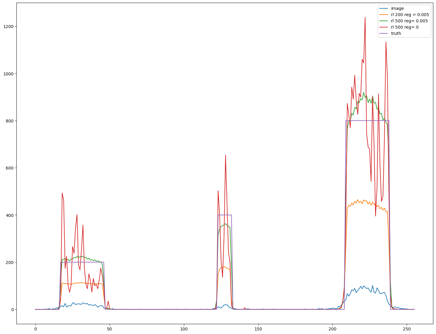
import matplotlib.pyplot as plt
s=im.shape

fig, ax = plt.subplots(figsize=(18,14))

line_z=int(s[0]//2)
line_y=int(7*s[1]//8)

line=im[line_z,line_y,:]
ax.plot(line, label = 'image')

line=decon1[line_z,line_y,:]
ax.plot(line, label='rl '+'200 reg = 0.005')

line=decon2[line_z,line_y,:]
ax.plot(line, label='rl '+'500 reg= 0.005')

line=decon3[line_z,line_y,:]
ax.plot(line, label='rl '+'500 reg= 0')

line=phantom[line_z,line_y,:]
ax.plot(line, label='truth')

ax.legend()
<matplotlib.legend.Legend at 0x1f84620c0a0>
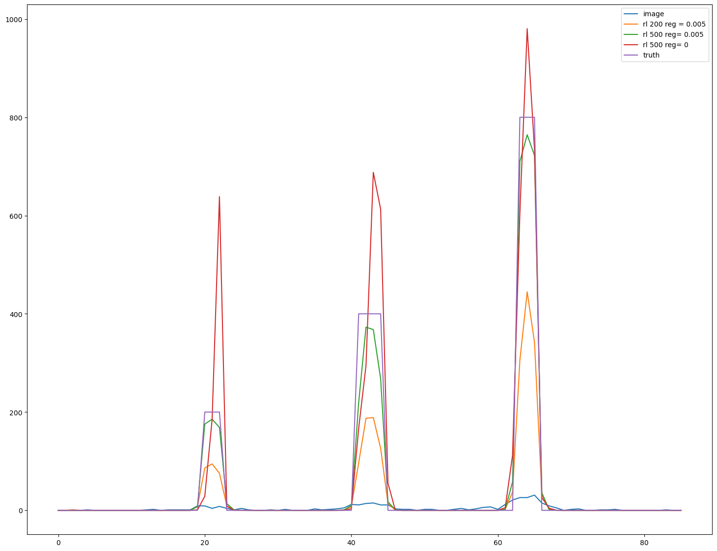
import matplotlib.pyplot as plt
s=im.shape

fig, ax = plt.subplots(figsize=(18,14))

line_y=int(s[1]//2)
line_x=int(s[1]//8)

line=im[:,line_y,line_x]
ax.plot(line, label = 'image')

line=decon1[:,line_y,line_x]
ax.plot(line, label='rl '+'200 reg = 0.005')

line=decon2[:,line_y,line_x]
ax.plot(line, label='rl '+'500 reg= 0.005')

line=decon3[:,line_y,line_x]
ax.plot(line, label='rl '+'500 reg= 0')

line=phantom[:,line_y,line_x]
ax.plot(line, label='truth')

ax.legend()
<matplotlib.legend.Legend at 0x1f845dd0970>
View in Napari#
import napari
viewer = napari.Viewer()
viewer.add_image(phantom, scale=[3,1,1],name='phantom')
viewer.add_image(im, scale=[3,1,1],name='im')
viewer.add_image(decon1, scale=[3,1,1],name='decon 1')
viewer.add_image(decon2, scale=[3,1,1],name='decon 2')
viewer.add_labels(labels_im, scale=[3,1,1],name='labels_im')
viewer.add_labels(labels_decon1, scale=[3,1,1],name='labels_decon 1')
viewer.add_labels(labels_decon2, scale=[3,1,1],name='labels_decon 2')
napari.manifest -> 'napari-hello' could not be imported: Cannot find module 'napari_plugins' declared in entrypoint: 'napari_plugins:napari.yaml'
<Labels layer 'labels_decon 2' at 0x1f89918ac70>
